Density Estimation

밀도 추정(Density Estimation)은 비지도 학습(Unsupervised Learning) 작업이다.

목표 : 주어진 데이터로부터 확률 질량 함수(PMF, Probability Mass Function) 또는 확률 밀도 함수(PDF, Probability Density Function) 를 학습하여 기본 확률 분포 모델을 추정하는 것.

 

Density Estimation 에 대한 개념을 익히기전, IID 는 꼭 기억하고 있어야 한다.

 

Standard(IID) assumtion 

Independent of each other

Coming from the same distribution 

indepenently identically distributed

 

Types

1. Parameteric : assuming a functional form of the distribution θ

• The distribution is modeled using a set of parameters θ

$$ \hat{p}(X) = p(X|θ) $$

• Estimation : Find parameters θ that is describe data D 
• E.g.: Mean and covariances of a multivariate Gaussian distribution
• Parametric statistic은 고정된 Parameter의 Set이 있는 확률분포로 모델링 할 수 있는 Population 으로부터 Sample data를 가져오는것으로 가정하는 Statistic의 한 분야이다

2. Nonparametric : no assumption about the underlying distribution

• The model of the distribution ustilizes all exmaples in D (estimate the density directly from the data) 
• E.g : Histogram, Kernel density estimaiton(KDE)
• 사전 정보 혹은 사전 지식 없이 즉, 데이터가 특정 분포를 따르는 가정이 없기 때문이  순수하게 Observation data ( 튜닝 parameter가 명확하지 않은 ) set으로만 PDF를 추정해야 하는 방식이다

 

 

Parametric Methods

Learning via Parameter estimation

• Assumption : There exist true values for parameters θ, however, the values are unkwon(estimation theory)
• Settings
  • Random variables X= {X_1,....,X_d)
  • A model of the distribution over variables X with parameters θ : p̂(X|θ)
  • Data D = {d_1,d_2... d_N}
• Objective : Find parameters θ such that p̂(X|θ) fits data D the best

MLE 

• A method of edstimating the parameters of a model 
• Works by maximizing a likelihood function ( the observed data will be most probalbe)
• Objective : θ that maximizes likelihood P(D|θ) 
• Under the IID assumption, the likelihood of D is 

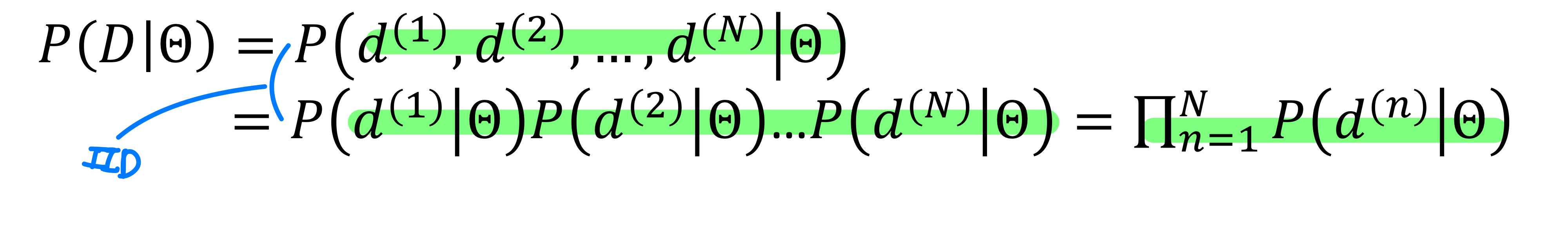
MLE 전개

 

• 아래와 같이 계속 확률을 곱해주면 값이 매우작아져서 log-likelihood 를 사용해서 표현

 

이러한 MLE 도 몇가지 단점이 있다. 

• MLE picks only one set of the parameter values.
  • 만약 두개의 파라미터가 cls in terms of the likelihood, 오직 하나의 파라미터만 사용하면 강한 바이어스를 생기게 할 수 있음 

그래서 이걸 해결하고자 Bayesian parameter estimation 을 사용 할 수 있음.

 

 

Bayesian parameter estimation 

• Remedies the limitation of one choice
• Uses the posterior distribution for parameters θ
• Posterior covers all possible parameter values (and weights)

Bayesian Prameter estimation : Prior on parameters θ + [Data + Mode P(X|θ)]  -> Posterior on Parameters θ

MLE  : No prior + [Data + Mode P(X|θ)] -> Just one set of parmeters value(θ)

두개의 방법은 차이가 있다.

 

1. MLE (Maximum Likelihood Estimation)
   • 주어진 데이터 X 에 대해, 우도 함수 P(X∣θ) 를 최대화하는 단 하나의 파라미터 θ값을 추정
   • 사전 정보(즉, Prior)를 고려하지 않고 오직 데이터만을 이용하여 최적의 θ 값을 찾는 방법
   • 즉, 최적의 하나의 파라미터 값을 찾음
2. Bayesian Parameter Estimation
   • MLE와 달리 사전 정보(Prior) 를 반영하여 파라미터를 추정
   • 사전 분포 P(θ) 와 우도 P(X∣θ) 를 결합하여 베이즈 정리를 통해 사후 분포 P(θ∣X) 를 계산
   • 결과적으로, 단 하나의 θ값이 아닌 사후 확률 분포(Post. Dist.) 를 얻을 수 있으며, 이로부터 여러 가지 방식(예: MAP 추정, 평균 등)으로 최적의 θ를 선택

즉, MLE는 단일 최적 값을 찾지만, 베이지안 추정은 사전 정보를 반영하여 확률적 분포를 기반으로 파라미터를 추정하는 차이가 있다.

 

 

 

다음은 다양한 분표 종류다. 아래 분포들에 대한 MLE 를 일일이 손으로 구해보면 MLE 가 더 마음에 와닿는다. 

 

Models for discrete random variables (finite number of outcomes)

• Bernoulli distribution : coin flip
• Binomial distribution : Tossing N coins with a fixed bias θ
• Multinomial distribution : Rolling dice N times
• Poisson distribution : The number of calls received by a customer call center per hour 
  • 단위 시간 혹은 단위 공간 안에 어떤 사건이 몇번 발생할 것인가를 표현한 확률 분포

 

Models for continuous random variables (infinitely many outcomes)

• Uniform distribution
• Gaussian distribution
• Gamma distribution
• Exponnetial distribution

 

Central Limit Theorem

• The sample mean will be approximately normally distributed for large sample sizes, regardless of the distribution from which we are sampling
• 모집단이 평균이 µ 이고 표준편차가 σ 인 임의의 분포를 이룰 때, 이 모집단으로 부터 추출된 표본의 크기(=n) 이 충분히 크다면, 표본들이 이루는 분포는 평균이 µ 이고 표준편차가 σ/√n 인 정규분포에 근접한다.
• 표본 분포와 모집단의 관계를 증명함으로써, 수집한 통계량을 이용하여, Parameter 를 추정할 수 있게 하는 확률적 근거
• E.g : Galton Board (feat. Bernoiulli trial)

Cramer's Theorem

Let a random variable X be normally distributed and decomposed as a sum of two independent random variable (X = X_1+X_2), then the summands X_1 and X_2 are also normally distributed  →

임의의 확률 변수 X가 정규 분포를 따르고, 이 변수를 두 개의 독립적인 확률 변수 X_1과 X_2 의 합으로 나타낼 수 있다고 하면 X_1과 X_2  모두 정규분포를 따름

 

Nonparmateric Density Estimation 

Histogram

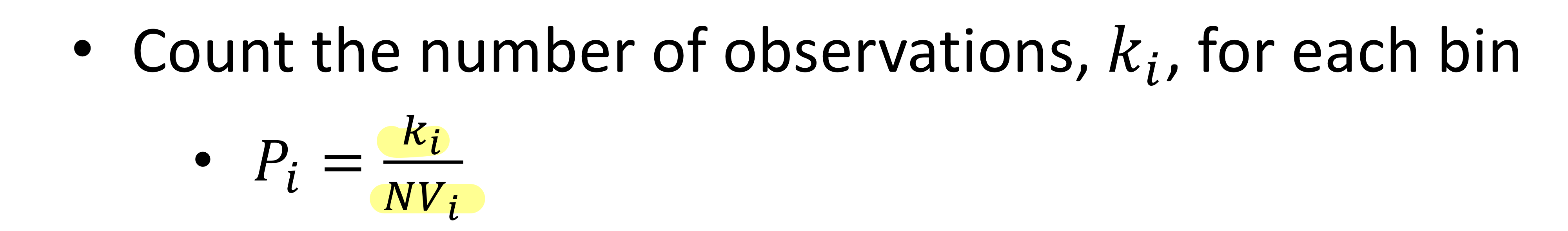
• Pack your data in some number of equally spaced intervals and count the data points falling into each interval 
• 데이터의 밀도를 간단한 형태로 표현 → 측정된 스케일로 이루어진 데이터를 연속적인 간격으로 나누고 각 간격에서 관측되는 표본의 빈도를 카운트하여 그 값을 막대의 높이로 하여 데이터의 밀도를 표현한 그래프 
• V : bin width 

 

Adavntage

• Conveys information about data faster than tables
• Gives more complete information about data

Issues

• Depending on the starting point
• Does not work well in a high-dimensional space

Solution

• Build a PDF P(x) by estimating how similar D are to x  (E.g., Parzen window method (KDE)
• →  동적으로 bins 을 조절 

 

KDE (kernel density estimation)

위에서 말했던 것 처럼 히스토그램 방법은 'bin의 경계에서 불연속성이 나타남','bin의 크기 및 시작 위치에 따라 히스토그램이 달라짐','고차원 데이터 메모리 문제' 의 문제가 있다.  이를 해결하고자 Kernel function 을 이용하여 히스토 그램 방법의 문제를 개선한다. 

 

Kernel function

• 원점을 중심으로 좌우 대칭이면서 (Symmetric)
• 적분 값이 1인 non-negative 함수
• E.g., Gaussian, uniform 함수 등이 대표적인 커널 함수 이다.

 

커널 함수와 KDE 시각화

구체적인 방법은 다음과 같다.

 

• 각 관측 데이터 포인트에 커널 함수 적용
  • 관측된 데이터 각각 마다 해당 데이터 값을 중심으로 하는 커널 함수를 x생성 : K(x-xi)
• 모든 데이터 포인트에서 생성된 커널 함수들을 합산
  • 각 데이터 포인트에서 얻어진 커널 값을 모두 더함
• 전체 데이터 개수 n과 h(bandwidth)로 정규화
  • 이렇게 만든 밀도 함수의 합을 전체 데이터 개수 n 로 나누어 확률 밀도로 변환
  • bandwidth h  를 사용하여 스무딩 효과를 조절

 

 

 

 

Ref

 

 

[개념 통계 17] 중심극한 정리는 무엇이고 왜 중요한가?

 

KDE -Kernel Density Estimation 이란 ?